Generally, Excel appears too good to be true. All I’ve to do is enter a formulation, and just about something I would ever must do manually might be performed robotically.

Have to merge two sheets with comparable knowledge? Excel can do it.

Have to do simple arithmetic? Excel can do it.

Want to mix data in a number of cells? Excel can do it.

On this submit, I’ll go over the perfect ideas, tips, and shortcuts you should utilize proper now to take your Excel recreation to the following stage. No superior Excel information required.

What’s Excel?

Microsoft Excel is highly effective knowledge visualization and evaluation software program, which makes use of spreadsheets to retailer, manage, and observe knowledge units with formulation and capabilities. Excel is utilized by entrepreneurs, accountants, knowledge analysts, and different professionals. It is a part of the Microsoft Workplace suite of merchandise. Options embody Google Sheets and Numbers. 

Discover extra Excel alternate options right here.

Excel is primarily used for creating monetary paperwork due to its sturdy computational powers. You’ll usually discover the software program in accounting workplaces and groups as a result of it permits accountants to robotically see sums, averages, and totals. With Excel, they’ll simply make sense of their enterprise’ knowledge.

Whereas Excel is primarily often called an accounting instrument, professionals in any subject can use its options and formulation — particularly entrepreneurs — as a result of it may be used for monitoring any kind of information. It removes the necessity to spend hours and hours counting cells or copying and pasting efficiency numbers. Excel usually has a shortcut or fast repair that hastens the method.

You can too obtain Excel templates under for your entire advertising wants. 

After you obtain the templates, it’s time to start out utilizing the software program. Let’s cowl the fundamentals first.

Excel Fundamentals

When you’re simply beginning out with Excel, there are a number of fundamental instructions that we recommend you develop into aware of. These are issues like:

• Creating a brand new spreadsheet from scratch.
• Executing fundamental computations like including, subtracting, multiplying, and dividing.
• Writing and formatting column textual content and titles.
• Utilizing Excel’s auto-fill options.
• Including or deleting single columns, rows, and spreadsheets. (Beneath, we’ll get into the way to add issues like a number of columns and rows.)
• Protecting column and row titles seen as you scroll previous them in a spreadsheet, in order that you already know what knowledge you are filling as you progress additional down the doc.
• Sorting your knowledge in alphabetical order. 

Let’s discover a number of of those extra in-depth. 

As an example, why does auto-fill matter? 

In case you have any fundamental Excel information, it’s doubtless you already know this fast trick. However to cowl our bases, enable me to point out you the glory of autofill. This allows you to shortly fill adjoining cells with a number of varieties of knowledge, together with values, collection, and formulation.

There are a number of methods to deploy this characteristic, however the fill deal with is among the many best. Choose the cells you wish to be the supply, find the fill deal with within the lower-right nook of the cell, and both drag the fill deal with to cowl cells you wish to fill or simply double click on:

Equally, sorting is a vital characteristic you may wish to know when organizing your knowledge in Excel. 

Generally you might have a listing of information that has no group in anyway. Perhaps you exported a listing of your advertising contacts or weblog posts. Regardless of the case could also be, Excel’s type characteristic will show you how to alphabetize any listing.

Click on on the info within the column you wish to type. Then click on on the “Information” tab in your toolbar and search for the “Kind” choice on the left. If the “A” is on prime of the “Z,” you possibly can simply click on on that button as soon as. If the “Z” is on prime of the “A,” click on on the button twice. When the “A” is on prime of the “Z,” which means your listing will likely be sorted in alphabetical order. Nonetheless, when the “Z” is on prime of the “A,” which means your listing will likely be sorted in reverse alphabetical order.

Let’s discover extra of the fundamentals of Excel (together with superior options) subsequent. 

Easy methods to Use Excel

To make use of Excel, you solely must enter the info into the rows and columns. And then you definately’ll use formulation and capabilities to show that knowledge into insights. 

We’ll go over the perfect formulation and capabilities you want to know. However first, let’s check out the varieties of paperwork you possibly can create utilizing the software program. That approach, you will have an overarching understanding of how you should utilize Excel in your day-to-day. 

Paperwork You Can Create in Excel

Undecided how one can really use Excel in your workforce? Here’s a listing of paperwork you possibly can create:

• Revenue Statements: You should use an Excel spreadsheet to trace an organization’s gross sales exercise and monetary well being.
• Stability Sheets: Stability sheets are among the many most typical varieties of paperwork you possibly can create with Excel. It means that you can get a holistic view of an organization’s monetary standing.
• Calendar: You’ll be able to simply create a spreadsheet month-to-month calendar to trace occasions or different date-sensitive data.

Listed here are some paperwork you possibly can create particularly for entrepreneurs.

That is solely a small sampling of the varieties of advertising and enterprise paperwork you possibly can create in Excel. We’ve created an intensive listing of Excel templates you should utilize proper now for advertising, invoicing, mission administration, budgeting, and extra.

Within the spirit of working extra effectively and avoiding tedious, handbook work, listed below are a number of Excel formulation and capabilities you’ll must know.

Excel Formulation

It’s straightforward to get overwhelmed by the wide selection of Excel formulation that you should utilize to make sense out of your knowledge. When you’re simply getting began utilizing Excel, you possibly can depend on the next formulation to hold out some complicated capabilities — with out including to the complexity of your studying path.

• Equal signal: Earlier than creating any formulation, you’ll want to jot down an equal signal (=) within the cell the place you need the outcome to look.
• Addition: So as to add the values of two or extra cells, use the + signal. Instance: =C5+D3.
• Subtraction: To subtract the values of two or extra cells, use the – signal. Instance: =C5-D3.
• Multiplication: To multiply the values of two or extra cells, use the * signal. Instance: =C5*D3.
• Division: To divide the values of two or extra cells, use the / signal. Instance: =C5/D3.

Placing all of those collectively, you possibly can create a formulation that provides, subtracts, multiplies, and divides multi functional cell. Instance: =(C5-D3)/((A5+B6)*3).

For extra complicated formulation, you’ll want to make use of parentheses across the expressions to keep away from by accident utilizing the PEMDAS order of operations. Take into account that you should utilize plain numbers in your formulation.

Excel Capabilities

Excel capabilities automate among the duties you’d use in a typical formulation. As an example, as a substitute of utilizing the + signal so as to add up a spread of cells, you’d use the SUM perform. Let’s have a look at a number of extra capabilities that can assist automate calculations and duties.

• SUM: The SUM perform robotically provides up a spread of cells or numbers. To finish a sum, you’d enter the beginning cell and the ultimate cell with a colon in between. Right here’s what that appears like: SUM(Cell1:Cell2). Instance: =SUM(C5:C30).
• AVERAGE: The AVERAGE perform averages out the values of a spread of cells. The syntax is similar because the SUM perform: AVERAGE(Cell1:Cell2). Instance: =AVERAGE(C5:C30).
• IF: The IF perform means that you can return values based mostly on a logical check. The syntax is as follows: IF(logical_test, value_if_true, [value_if_false]). Instance: =IF(A2>B2,”Over Finances”,”OK”).
• VLOOKUP: The VLOOKUP perform helps you seek for something in your sheet’s rows. The syntax is: VLOOKUP(lookup worth, desk array, column quantity, Approximate match (TRUE) or Precise match (FALSE)). Instance: =VLOOKUP([@Attorney],tbl_Attorneys,4,FALSE).
• INDEX: The INDEX perform returns a worth from inside a spread. The syntax is as follows: INDEX(array, row_num, [column_num]).
• MATCH: The MATCH perform seems to be for a sure merchandise in a spread of cells and returns the place of that merchandise. It may be utilized in tandem with the INDEX perform. The syntax is: MATCH(lookup_value, lookup_array, [match_type]).
• COUNTIF: The COUNTIF perform returns the variety of cells that meet a sure standards or have a sure worth. The syntax is: COUNTIF(vary, standards). Instance: =COUNTIF(A2:A5,”London”).

Okay, able to get into the nitty-gritty? Let’s get to it. (And to all of the Harry Potter followers on the market … you are welcome upfront.)

Notice: The GIFs and visuals are from a earlier model of Excel. When relevant, the copy has been up to date to offer instruction for customers of each newer and older Excel variations.

1. Use Pivot tables to acknowledge and make sense of information.

Pivot tables are used to reorganize knowledge in a spreadsheet. They will not change the info that you’ve got, however they’ll sum up values and examine totally different data in your spreadsheet, relying on what you need them to do.

Let’s check out an instance. To illustrate I need to check out how many individuals are in every home at Hogwarts. It’s possible you’ll be pondering that I haven’t got an excessive amount of knowledge, however for longer knowledge units, it will turn out to be useful.

To create the Pivot Desk, I’m going to Information > Pivot Desk. When you’re utilizing the latest model of Excel, you’d go to Insert > Pivot Desk. Excel will robotically populate your Pivot Desk, however you possibly can all the time change across the order of the info. Then, you will have 4 choices to select from.

• Report Filter: This lets you solely have a look at sure rows in your dataset. For instance, if I wished to create a filter by home, I may select to solely embody college students in Gryffindor as a substitute of all college students.
• Column Labels: These can be your headers within the dataset.
• Row Labels: These might be your rows within the dataset. Each Row and Column labels can include knowledge out of your columns (e.g. First Identify might be dragged to both the Row or Column label — it simply is dependent upon the way you wish to see the info.)
• Worth: This part means that you can have a look at your knowledge in a different way. As a substitute of simply pulling in any numeric worth, you possibly can sum, rely, common, max, min, rely numbers, or do a number of different manipulations along with your knowledge. In reality, by default, if you drag a subject to Worth, it all the time does a rely.

Since I wish to rely the variety of college students in every home, I will go to the Pivot desk builder and drag the Home column to each the Row Labels and the Values. It will sum up the variety of college students related to every home.

2. Add a couple of row or column.

As you mess around along with your knowledge, you may discover you are always needing so as to add extra rows and columns. Generally, you might even want so as to add tons of of rows. Doing this one-by-one can be tremendous tedious. Fortunately, there’s all the time a better approach.

So as to add a number of rows or columns in a spreadsheet, spotlight the identical variety of preexisting rows or columns that you just wish to add. Then, right-click and choose “Insert.”

Within the instance under, I wish to add a further three rows. By highlighting three rows after which clicking insert, I can add a further three clean rows into my spreadsheet shortly and simply.

3. Use filters to simplify your knowledge.

If you’re very massive knowledge units, you do not normally have to be each single row on the identical time. Generally, you solely wish to have a look at knowledge that match into sure standards.

That is the place filters are available in.

Filters can help you pare down your knowledge to solely have a look at sure rows at one time. In Excel, a filter might be added to every column in your knowledge — and from there, you possibly can then select which cells you wish to view without delay.

Let’s check out the instance under. Add a filter by clicking the Information tab and choosing “Filter.” Clicking the arrow subsequent to the column headers and you’ll select whether or not you need your knowledge to be organized in ascending or descending order, in addition to which particular rows you wish to present.

In my Harry Potter instance, for example I solely wish to see the scholars in Gryffindor. By choosing the Gryffindor filter, the opposite rows disappear.

Professional Tip: Copy and paste the values within the spreadsheet when a Filter is on to do further evaluation in one other spreadsheet.

4. Take away duplicate knowledge factors or units.

Bigger knowledge units are likely to have duplicate content material. You will have a listing of a number of contacts in an organization and solely wish to see the variety of corporations you will have. In conditions like this, eradicating the duplicates is available in fairly useful.

To take away your duplicates, spotlight the row or column that you just wish to take away duplicates of. Then, go to the Information tab and choose “Take away Duplicates” (which is below the Instruments subheader within the older model of Excel). A pop-up will seem to verify which knowledge you wish to work with. Choose “Take away Duplicates,” and also you’re good to go.

You can too use this characteristic to take away a complete row based mostly on a reproduction column worth. So you probably have three rows with Harry Potter’s data and also you solely must see one, then you possibly can choose the entire dataset after which take away duplicates based mostly on e mail. Your ensuing listing could have solely distinctive names with none duplicates.

5. Transpose rows into columns.

When you will have rows of information in your spreadsheet, you may determine you really wish to rework the gadgets in a type of rows into columns (or vice versa). It might take a variety of time to repeat and paste every particular person header — however what the transpose characteristic means that you can do is solely transfer your row knowledge into columns, or the opposite approach round.

Begin by highlighting the column that you just wish to transpose into rows. Proper-click it, after which choose “Copy.” Subsequent, choose the cells in your spreadsheet the place you need your first row or column to start. Proper-click on the cell, after which choose “Paste Particular.” A module will seem — on the backside, you may see an choice to transpose. Examine that field and choose OK. Your column will now be transferred to a row or vice-versa.

On newer variations of Excel, a drop-down will seem as a substitute of a pop-up.

6. Cut up up textual content data between columns.

What if you wish to break up out data that is in a single cell into two totally different cells? For instance, perhaps you wish to pull out somebody’s firm identify by way of their e mail deal with. Or maybe you wish to separate somebody’s full identify into a primary and final identify to your e mail advertising templates.

Because of Excel, each are attainable. First, spotlight the column that you just wish to break up up. Subsequent, go to the Information tab and choose “Textual content to Columns.” A module will seem with further data.

First, you want to choose both “Delimited” or “Fastened Width.”

• “Delimited” means you wish to break up the column based mostly on characters akin to commas, areas, or tabs.
• “Fastened Width” means you wish to choose the precise location on all of the columns that you really want the break up to happen.

Within the instance case under, let’s choose “Delimited” so we are able to separate the complete identify into first identify and final identify.

Then, it is time to decide on the Delimiters. This might be a tab, semi-colon, comma, house, or one thing else. (“One thing else” might be the “@” signal utilized in an e mail deal with, for instance.) In our instance, let’s select the house. Excel will then present you a preview of what your new columns will seem like.

If you’re proud of the preview, press “Subsequent.” This web page will can help you choose Superior Codecs when you select to. If you’re performed, click on “End.”

7. Use formulation for easy calculations.

Along with doing fairly complicated calculations, Excel can assist you do easy arithmetic like including, subtracting, multiplying, or dividing any of your knowledge.

• So as to add, use the + signal.
• To subtract, use the – signal.
• To multiply, use the * signal.
• To divide, use the / signal.

You can too use parentheses to make sure sure calculations are performed first. Within the instance under (10+10*10), the second and third 10 have been multiplied collectively earlier than including the extra 10. Nonetheless, if we made it (10+10)*10, the primary and second 10 can be added collectively first.

8. Get the common of numbers in your cells.

If you’d like the common of a set of numbers, you should utilize the formulation =AVERAGE(Cell1:Cell2). If you wish to sum up a column of numbers, you should utilize the formulation =SUM(Cell1:Cell2).

9. Use conditional formatting to make cells robotically change colour based mostly on knowledge.

Conditional formatting means that you can change a cell’s colour based mostly on the data inside the cell. For instance, if you wish to flag sure numbers which can be above common or within the prime 10% of the info in your spreadsheet, you are able to do that. If you wish to colour code commonalities between totally different rows in Excel, you are able to do that. It will show you how to shortly see data that’s necessary to you.

To get began, spotlight the group of cells you wish to use conditional formatting on. Then, select “Conditional Formatting” from the House menu and choose your logic from the dropdown. (You can too create your personal rule if you would like one thing totally different.) A window will pop up that prompts you to offer extra details about your formatting rule. Choose “OK” if you’re performed, and it is best to see your outcomes robotically seem.

10. Use the IF Excel formulation to automate sure Excel capabilities.

Generally, we do not wish to rely the variety of instances a worth seems. As a substitute, we wish to enter totally different data right into a cell if there’s a corresponding cell with that data.

For instance, within the state of affairs under, I wish to award ten factors to everybody who belongs within the Gryffindor home. As a substitute of manually typing in 10’s subsequent to every Gryffindor scholar’s identify, I can use the IF Excel formulation to say that if the coed is in Gryffindor, then they need to get ten factors.

The formulation is: IF(logical_test, value_if_true, [value_if_false])

Instance Proven Beneath: =IF(D2=”Gryffindor”,”10″,”0″)

Generally phrases, the formulation can be IF(Logical Check, worth of true, worth of false). Let’s dig into every of those variables.

• Logical_Test: The logical check is the “IF” a part of the assertion. On this case, the logic is D2=”Gryffindor” as a result of we wish to make it possible for the cell corresponding with the coed says “Gryffindor.” Be certain to place Gryffindor in citation marks right here.
• Value_if_True: That is what we would like the cell to point out if the worth is true. On this case, we would like the cell to point out “10” to point that the coed was awarded the ten factors. Solely use citation marks if you would like the outcome to be textual content as a substitute of a quantity.
• Value_if_False: That is what we would like the cell to point out if the worth is fake. On this case, for any scholar not in Gryffindor, we would like the cell to point out “0”. Solely use citation marks if you would like the outcome to be textual content as a substitute of a quantity.

Notice: Within the instance above, I awarded 10 factors to everybody in Gryffindor. If I later wished to sum the overall variety of factors, I would not be capable to as a result of the ten’s are in quotes, thus making them textual content and never a quantity that Excel can sum.

The true energy of the IF perform comes if you string a number of IF statements collectively, or nest them. This lets you set a number of circumstances, get extra particular outcomes, and in the end manage your knowledge into extra manageable chunks.

Ranges are one strategy to phase your knowledge for higher evaluation. For instance, you possibly can categorize knowledge into values which can be lower than 10, 11 to 50, or 51 to 100. Here is how that appears in apply: 

=IF(B3<11,“10 or much less”,IF(B3<51,“11 to 50”,IF(B3<100,“51 to 100”)))

It could take some trial-and-error, however after you have the grasp of it, IF formulation will develop into your new Excel greatest good friend.

11. Use greenback indicators to maintain one cell’s formulation the identical no matter the place it strikes.

Have you ever ever seen a greenback register an Excel formulation? When utilized in a formulation, it is not representing an American greenback; as a substitute, it makes positive that the precise column and row are held the identical even when you copy the identical formulation in adjoining rows.

You see, a cell reference — if you seek advice from cell A5 from cell C5, for instance — is relative by default. In that case, you are really referring to a cell that is 5 columns to the left (C minus A) and in the identical row (5). That is referred to as a relative formulation. If you copy a relative formulation from one cell to a different, it will modify the values within the formulation based mostly on the place it is moved. However typically, we would like these values to remain the identical regardless of whether or not they’re moved round or not — and we are able to try this by turning the formulation into an absolute formulation.

To vary the relative formulation (=A5+C5) into an absolute formulation, we might precede the row and column values by greenback indicators, like this: (=$A$5+$C$5). (Be taught extra on Microsoft Workplace’s assist web page right here.)

12. Use the VLOOKUP perform to tug knowledge from one space of a sheet to a different.

Have you ever ever had two units of information on two totally different spreadsheets that you just wish to mix right into a single spreadsheet?

For instance, you might need a listing of individuals’s names subsequent to their e mail addresses in a single spreadsheet, and a listing of those self same folks’s e mail addresses subsequent to their firm names within the different — however you need the names, e mail addresses, and firm names of these folks to look in a single place.

I’ve to mix knowledge units like this loads — and after I do, the VLOOKUP is my go-to formulation.

Earlier than you utilize the formulation, although, be completely positive that you’ve got not less than one column that seems identically in each locations. Scour your knowledge units to verify the column of information you are utilizing to mix your data is precisely the identical, together with no further areas.

The formulation: =VLOOKUP(lookup worth, desk array, column quantity, Approximate match (TRUE) or Precise match (FALSE))

The formulation with variables from our instance under: =VLOOKUP(C2,Sheet2!A:B,2,FALSE)

On this formulation, there are a number of variables. The next is true if you wish to mix data in Sheet 1 and Sheet 2 onto Sheet 1.

• Lookup Worth: That is the an identical worth you will have in each spreadsheets. Select the primary worth in your first spreadsheet. Within the instance that follows, this implies the primary e mail deal with on the listing, or cell 2 (C2).
• Desk Array: The desk array is the vary of columns on Sheet 2 you are going to pull your knowledge from, together with the column of information an identical to your lookup worth (in our instance, e mail addresses) in Sheet 1 in addition to the column of information you are attempting to repeat to Sheet 1. In our instance, that is “Sheet2!A:B.” “A” means Column A in Sheet 2, which is the column in Sheet 2 the place the info an identical to our lookup worth (e mail) in Sheet 1 is listed. The “B” means Column B, which accommodates the data that is solely obtainable in Sheet 2 that you just wish to translate to Sheet 1.
• Column Quantity: This tells Excel which column the brand new knowledge you wish to copy to Sheet 1 is situated in. In our instance, this is able to be the column that “Home” is situated in. “Home” is the second column in our vary of columns (desk array), so our column quantity is 2. [Note: Your range can be more than two columns. For example, if there are three columns on Sheet 2 — Email, Age, and House — and you still want to bring House onto Sheet 1, you can still use a VLOOKUP. You just need to change the “2” to a “3” so it pulls back the value in the third column: =VLOOKUP(C2:Sheet2!A:C,3,false).]
• Approximate Match (TRUE) or Precise Match (FALSE): Use FALSE to make sure you pull in solely precise worth matches. When you use TRUE, the perform will pull in approximate matches.

Within the instance under, Sheet 1 and Sheet 2 include lists describing totally different details about the identical folks, and the widespread thread between the 2 is their e mail addresses. To illustrate we wish to mix each datasets so that every one the home data from Sheet 2 interprets over to Sheet 1.

So after we kind within the formulation =VLOOKUP(C2,Sheet2!A:B,2,FALSE), we deliver all the home knowledge into Sheet 1.

Take into account that VLOOKUP will solely pull again values from the second sheet which can be to the proper of the column containing your an identical knowledge. This could result in some limitations, which is why some folks desire to make use of the INDEX and MATCH capabilities as a substitute.

13. Use INDEX and MATCH formulation to tug knowledge from horizontal columns.

Like VLOOKUP, the INDEX and MATCH capabilities pull in knowledge from one other dataset into one central location. Listed here are the primary variations:

• VLOOKUP is a a lot less complicated formulation. When you’re working with massive knowledge units that will require 1000’s of lookups, utilizing the INDEX and MATCH perform will considerably lower load time in Excel.
• The INDEX and MATCH formulation work right-to-left, whereas VLOOKUP formulation solely work as a left-to-right lookup. In different phrases, if you want to do a lookup that has a lookup column to the proper of the outcomes column, then you definately’d should rearrange these columns with a view to do a VLOOKUP. This may be tedious with massive datasets and/or result in errors.

So if I wish to mix data in Sheet 1 and Sheet 2 onto Sheet 1, however the column values in Sheets 1 and a couple of aren’t the identical, then to do a VLOOKUP, I would want to change round my columns. On this case, I would select to do an INDEX and MATCH as a substitute.

Let us take a look at an instance. To illustrate Sheet 1 accommodates a listing of individuals’s names and their Hogwarts e mail addresses, and Sheet 2 accommodates a listing of individuals’s e mail addresses and the Patronus that every scholar has. (For the non-Harry Potter followers on the market, each witch or wizard has an animal guardian referred to as a “Patronus” related to her or him.) The knowledge that lives in each sheets is the column containing e mail addresses, however this e mail deal with column is in several column numbers on every sheet. I would use the INDEX and MATCH formulation as a substitute of VLOOKUP so I would not have to change any columns round.

So what is the formulation, then? The formulation is definitely the MATCH formulation nested contained in the INDEX formulation. You will see I differentiated the MATCH formulation utilizing a distinct colour right here.

The formulation: =INDEX(desk array, MATCH formulation)

This turns into: =INDEX(desk array, MATCH (lookup_value, lookup_array))

The formulation with variables from our instance under: =INDEX(Sheet2!A:A,(MATCH(Sheet1!C:C,Sheet2!C:C,0)))

Listed here are the variables:

• Desk Array: The vary of columns on Sheet 2 containing the brand new knowledge you wish to deliver over to Sheet 1. In our instance, “A” means Column A, which accommodates the “Patronus” data for every individual.
• Lookup Worth: That is the column in Sheet 1 that accommodates an identical values in each spreadsheets. Within the instance that follows, this implies the “e mail” column on Sheet 1, which is Column C. So: Sheet1!C:C.
• Lookup Array: That is the column in Sheet 2 that accommodates an identical values in each spreadsheets. Within the instance that follows, this refers back to the “e mail” column on Sheet 2, which occurs to even be Column C. So: Sheet2!C:C.

Upon getting your variables straight, kind within the INDEX and MATCH formulation within the top-most cell of the clean Patronus column on Sheet 1, the place you need the mixed data to reside.

14. Use the COUNTIF perform to make Excel rely phrases or numbers in any vary of cells.

As a substitute of manually counting how usually a sure worth or quantity seems, let Excel do the be just right for you. With the COUNTIF perform, Excel can rely the variety of instances a phrase or quantity seems in any vary of cells.

For instance, for example I wish to rely the variety of instances the phrase “Gryffindor” seems in my knowledge set.

The formulation: =COUNTIF(vary, standards)

The formulation with variables from our instance under: =COUNTIF(D:D,”Gryffindor”)

On this formulation, there are a number of variables:

• Vary: The vary that we would like the formulation to cowl. On this case, since we’re solely specializing in one column, we use “D:D” to point that the primary and final column are each D. If I have been columns C and D, I’d use “C:D.”
• Standards: No matter quantity or piece of textual content you need Excel to rely. Solely use citation marks if you would like the outcome to be textual content as a substitute of a quantity. In our instance, the standards is “Gryffindor.”

Merely typing within the COUNTIF formulation in any cell and urgent “Enter” will present me what number of instances the phrase “Gryffindor” seems within the dataset.

15. Mix cells utilizing &.

Databases have a tendency to separate out knowledge to make it as precise as attainable. For instance, as a substitute of getting a column that reveals an individual’s full identify, a database might need the info as a primary identify after which a final identify in separate columns. Or, it might have an individual’s location separated by metropolis, state, and zip code. In Excel, you possibly can mix cells with totally different knowledge into one cell through the use of the “&” register your perform.

The formulation with variables from our instance under: =A2&” “&B2

Let’s undergo the formulation collectively utilizing an instance. Fake we wish to mix first names and final names into full names in a single column. To do that, we might first put our cursor within the clean cell the place we would like the complete identify to look. Subsequent, we might spotlight one cell that accommodates a primary identify, kind in an “&” signal, after which spotlight a cell with the corresponding final identify.

However you are not completed — if all you kind in is =A2&B2, then there is not going to be an area between the individual’s first identify and final identify. So as to add that needed house, use the perform =A2&” “&B2. The citation marks across the house inform Excel to place an area in between the primary and final identify.

To make this true for a number of rows, merely drag the nook of that first cell downward as proven within the instance.

16. Add checkboxes.

When you’re utilizing an Excel sheet to trace buyer knowledge and wish to oversee one thing that is not quantifiable, you could possibly insert checkboxes right into a column.

For instance, when you’re utilizing an Excel sheet to handle your gross sales prospects and wish to observe whether or not you referred to as them within the final quarter, you could possibly have a “Known as this quarter?” column and examine off the cells in it if you’ve referred to as the respective consumer.

Here is the way to do it.

Spotlight a cell you need so as to add checkboxes to in your spreadsheet. Then, click on DEVELOPER. Then, below FORM CONTROLS, click on the checkbox or the choice circle highlighted within the picture under.

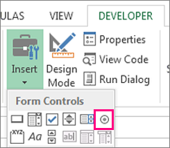
As soon as the field seems within the cell, copy it, spotlight the cells you additionally need it to look in, after which paste it.

17. Hyperlink a cell to a web site.

When you’re utilizing your sheet to trace social media or web site metrics, it may be useful to have a reference column with the hyperlinks every row is monitoring. When you add a URL instantly into Excel, it ought to robotically be clickable. However, if you must hyperlink phrases, akin to a web page title or the headline of a submit you are monitoring, this is how.

Spotlight the phrases you wish to hyperlink, then press Shift Ok. From there a field will pop up permitting you to put the hyperlink URL. Copy and paste the URL into this field and hit or click on Enter.

If the important thing shortcut is not working for any purpose, you may also do that manually by highlighting the cell and clicking Insert > Hyperlink.

18. Add drop-down menus.

Generally, you may be utilizing your spreadsheet to trace processes or different qualitative issues. Quite than writing phrases into your sheet repetitively, akin to “Sure”, “No”, “Buyer Stage”, “Gross sales Lead”, or “Prospect”, you should utilize dropdown menus to shortly mark descriptive issues about your contacts or no matter you are monitoring.

Here is the way to add drop-downs to your cells.

Spotlight the cells you need the drop-downs to be in, then click on the Information menu within the prime navigation and press Validation.

From there, you may see a Information Validation Settings field open. Have a look at the Enable choices, then click on Lists and choose Drop-down Listing. Examine the In-Cell dropdown button, then press OK.

19. Use the format painter. 

As you’ve most likely seen, Excel has a variety of options to make crunching numbers and analyzing your knowledge fast and simple. However when you ever spent a while formatting a sheet to your liking, you already know it could get a bit tedious.

Don’t waste time repeating the identical formatting instructions again and again. Use the format painter to simply copy the formatting from one space of the worksheet to a different. To take action, select the cell you’d like to duplicate, then choose the format painter choice (paintbrush icon) from the highest toolbar.

Excel Keyboard Shortcuts 

Creating reviews in Excel is time-consuming sufficient. How can we spend much less time navigating, formatting, and choosing gadgets in our spreadsheet? Glad you requested. There are a ton of Excel shortcuts on the market, together with a few of our favorites listed under.

Create a New Workbook

PC: Ctrl-N | Mac: Command-N

Choose Complete Row

PC: Shift-Area | Mac: Shift-Area

Choose Complete Column

PC: Ctrl-Area | Mac: Management-Area

Choose Remainder of Column

PC: Ctrl-Shift-Down/Up | Mac: Command-Shift-Down/Up

Choose Remainder of Row

PC: Ctrl-Shift-Proper/Left | Mac: Command-Shift-Proper/Left

Add Hyperlink

PC: Ctrl-Ok | Mac: Command-Ok

Open Format Cells Window

PC: Ctrl-1 | Mac: Command-1

Autosum Chosen Cells

PC: Alt-= | Mac: Command-Shift-T

Different Excel Assist Assets

Use Excel to Automate Processes in Your Staff

Even when you’re not an accountant, you possibly can nonetheless use Excel to automate duties and processes in your workforce. With the ideas and tips we shared on this submit, you’ll you should definitely use Excel to its fullest extent and get probably the most out of the software program to develop what you are promoting.

Editor’s Notice: This submit was initially printed in August 2017 however has been up to date for comprehensiveness.