Excel is an extremely highly effective software program – if you know the way to leverage it. With so many features and formulation choices, there’s one thing new to be taught each day.

The INDEX/MATCH formulation may help you discover information factors shortly with out having to manually seek for them and threat making errors.

Let’s dive into how that formulation works and evaluation some useful use circumstances.

Understanding INDEX and MATCH Capabilities Individually

Earlier than you possibly can perceive the way to use the INDEX and match formulation, it’s helpful to understand how every perform works by itself. That may provide some readability on how each work collectively as soon as mixed.

The INDEX perform returns a worth or the reference to a worth inside a desk or vary based mostly on the rows and columns you specify. Consider this perform as a GPS – it helps you discover information inside a doc however first, you must slim down the search space utilizing rows and columns.

The MATCH perform identifies a selected merchandise in a spread of cells then returns the relative place of that merchandise within the vary or the precise match.

For example, say the vary A1:A4 incorporates the values 15, 28, 49, 90. You wish to understand how the quantity “49” is relative to all values throughout the vary. You’ll write the formulation =MATCH(49,A1:A4,0) and it might return the quantity 3 as a result of it’s the third quantity within the vary. The 0 within the formulation represents “precise match.”

Now that we’ve bought the fundamentals out of the best way, let’s get into the way to mix the formulation and use it for a number of standards.

How one can Use the INDEX and MATCH Method with A number of Standards

The formulation for the INDEX/MATCH formulation is as follows: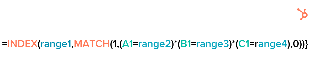

Right here’s how every perform works collectively: Match finds a worth and offers you its location. It then feeds that info to the INDEX perform, which turns that info right into a end result.

To see it in motion, let’s use an instance.

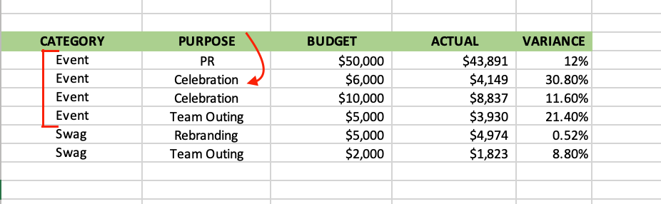
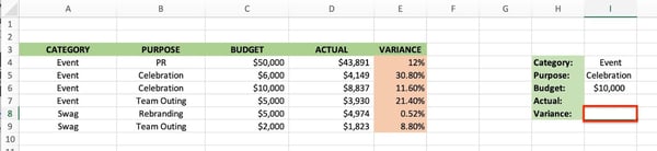
This Excel sheet includes a advertising and marketing finances for 2 classes: Occasions and firm swag presents. There are 4 functions: Public relations (PR), celebration, staff outing, and rebranding. The sheet additionally contains the outlined finances and the precise expense for every class.

That is the place the INDEX and MATCH formulation turns out to be useful when utilizing it for a number of standards. You’ll be able to shortly discover the reply(s) you’re on the lookout for and restrict errors that may occur when looking out manually.

Say you wish to know the variance for an occasion that had a function of celebration with a finances of 10,000 – right here’s the way you’d do it.

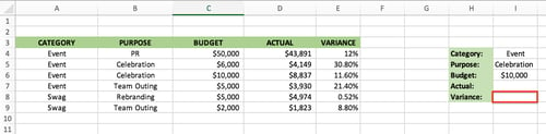
First, be aware of the row numbers and columns. The reply you’re on the lookout for will go in I8. Right here’s how the formulation will look:

Let’s break down the way you get there.

1. Create a separate part to jot down out your standards.

Step one on this course of is by itemizing out your standards and the determine you are on the lookout for someplace in your sheet. You will want this part later to create your formulation.

2. Begin with the INDEX.

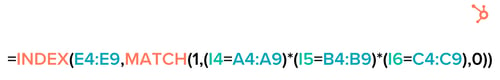
The formulation begins along with your GPS, which is the INDEX perform. You’re on the lookout for the variance, so you choose rows E4 by way of E9, as that’s the place the reply will probably be.

3. Add your ranges.

The extra columns you’ve got, the extra ranges you’ll want so as to add to slim down your outcomes.

As a reminder, you’re on the lookout for the variance for an occasion that had a $10,000 finances and had a function of celebration. Which means you’ll have to inform Excel which rows maintain the

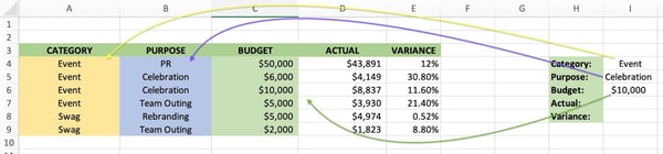
Beginning with the “occasion,” standards, you discover it first in I4., with its vary positioned in column A between rows 4 and 9.

Comply with the identical course of for “celebration” – it’s in I5 and its vary is B4 and B9. Lastly, the “$10,000” is in I6, with a spread of C4 by way of C9.

The final step right here is so as to add 0, which suggests you’re on the lookout for an actual match.

That’s how you find yourself with this last formulation:

4. Run the formulation.

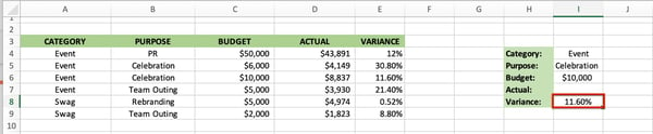
As a result of that is an array formulation, you will need to press Ctrl+Shift+Enter to get the fitting outcomes, except you’re utilizing Excel 365.

There you’ve got it!