Conditional formatting is a characteristic in Google Sheets wherein a cell is formatted in a selected method when sure circumstances are met. The formatting can embrace highlighting, bolding, italicizing – nearly any visible adjustments to the cell.

Simply as it may be completed for the cell you’re at present in, conditional formatting may also be set based mostly on circumstances met in one other cell.

Let’s dive into the way to create this situation based mostly on a number of standards.

How Conditional Formatting Works

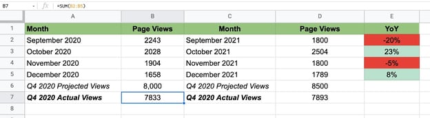
To learn to set conditional formatting, let’s use this workbook for example.

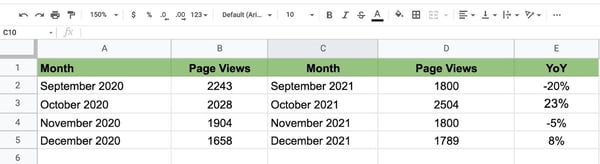
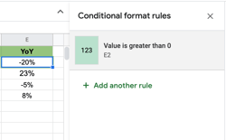
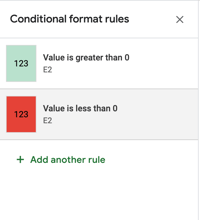
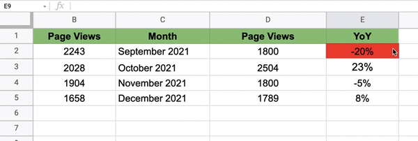
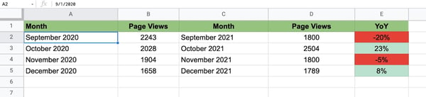
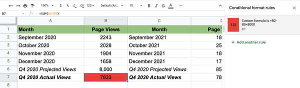
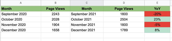
It’s a workbook displaying web site site visitors 12 months over 12 months from This autumn 2020 to This autumn 2021, with the web page views together with the year-over-year share change.

Right here’s what we need to accomplish right here: When the proportion change is optimistic YoY, the cell turns inexperienced. When it’s adverse, the cell turns purple. This makes it simple to get a fast efficiency overview earlier than diving into the small print.

Listed below are the steps to set the conditional formatting.

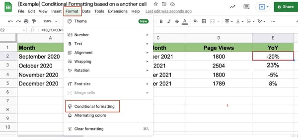
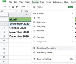
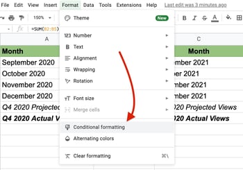
1. Choose the cell you need to format, click on on “Format” from the navigation bar, then click on on “Conditional Formatting.”

2. Whereas staying within the “Single shade” tab, double-check that the cell beneath “Apply to vary” is the cell you need to format.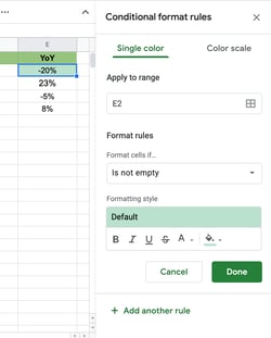

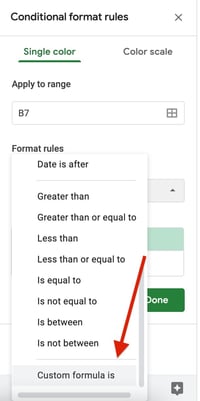
3. Set your format guidelines.

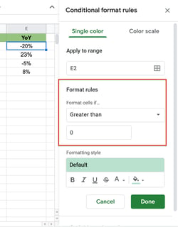
It could mechanically default to a typical conditional formatting system. On this case, open the dropdown menu beneath “Format cells if…” to pick your guidelines. Choices will look as follows:

4. Select your formatting fashion, then click on “Executed.”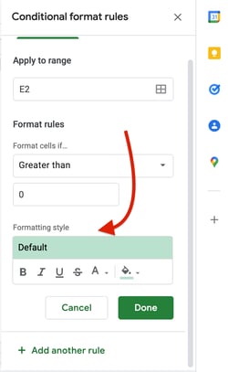

5. Affirm the rule was utilized beneath “Conditional Formatting Guidelines.”

6. Add one other rule if wanted.

7. Return to cell to view formatting, then drag the cursor to use to different cells, if wanted.

Now that you simply perceive the fundamentals, let’s cowl the way to use conditional formatting based mostly on different cells.

Conditional Formatting Primarily based on One other Cell Worth

1. Choose the cell you need to format.

2. Click on on “Format” within the navigation bar, then choose “Conditional Formatting.”

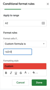
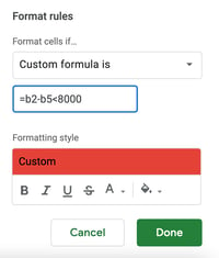
3. Below “Format Guidelines,” choose “Customized system is.”

4. Write your system, then click on “Executed.”

5. Affirm your rule has been utilized and examine the cell.

Conditional Formatting Primarily based on One other Cell Vary

To format based mostly on one other cell vary, you comply with most of the identical steps you’ll for a cell worth. What adjustments is the system you write.

1. Choose the cell you need to format.

2. Click on on “Format” within the navigation bar, then choose “Conditional Formatting.”

3. Below “Format Guidelines,” choose “Customized system is.”

4. Write your system utilizing the next format: =worth vary < [value], choose your formatting fashion, then click on “Executed.”

5. Affirm your rule has been utilized and examine the cell.

Google Sheets Conditional Formatting Based on Another Cell Color

Currently, Google Sheets does not offer a way to use conditional formatting based on the color of another cell. You can only use it based on:

• Values – higher than, greater than, equal to, in between
• Text – contains, starts with, ends with, matches
• Dates – is before, is after, is exactly
• Emptiness – is empty, is not empty

To achieve your goal, you’d have to use the condition of the cell to format the other.

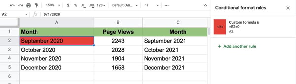
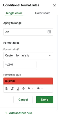
Let’s use an example.

Say you want to format cell A2 (September 2020) to be red and match the color of cell E2 (-20%). There’s no formula that allows you to create a condition based on color. However, you can create a custom formula based on E2’s values.

You can say that if cell E2’s values are less than 0, cell A2 turns red. The formula is as follows: = [The other cell] < [value]. On this case, the system can be =e2<0, because it signifies that cell A2 ought to flip purple if E2’s worth is lower than 0.

With so many features to play with, Google Sheets can appear daunting. By following these easy steps, you may simply format your cells for fast scanning.